The least squares method (least squares) is in the field of regression analysis. It has many uses, as it allows an approximate representation of a given function by other simpler ones. OLS can be extremely useful in processing observations, and it is actively used to estimate some values from the results of measurements of others containing random errors. In this article, you'll learn how to implement least squares calculations in Excel.
Statement of the problem on a concrete example
Suppose there are two indicators X and Y. Moreover, Y depends on X. Since MNCs are of interest to us from the point of view of regression analysis (in Excel its methods are implemented using built-in functions), we should immediately proceed to consider a specific problem.
So, let X be the sales area of the grocery store, measured in square meters, and Y the annual turnover, defined in millions of rubles.
It is required to make a forecast what kind of goods turnover (Y) the store will have if it has one or another retail space. Obviously, the function Y = f (X) is increasing, since the hypermarket sells more goods than the stall.
A few words about the correctness of the source data used for prediction
Suppose we have a table built according to data for n stores.
X | x 1 | x 2 | ... | x n |
Y | y 1 | y 2 | ... | y n |
According to mathematical statistics, the results will be more or less correct if the data on at least 5-6 objects are examined. In addition, “abnormal” results cannot be used. In particular, an elite small boutique can have turnover many times greater than the turnover of large retail outlets of the “masmarket” class.
The essence of the method
The table data can be represented on the Cartesian plane as points M 1 (x 1 , y 1 ), ... M n (x n , y n ). Now the solution of the problem is reduced to the selection of the approximating function y = f (x), which has a graph passing as close as possible to the points M 1, M 2, .. M n .
Of course, it is possible to use a polynomial of a high degree, but this option is not only difficult to implement, but simply incorrect, as it will not reflect the main trend that needs to be detected. The most reasonable solution is to find the straight line y = ax + b, which best approximates the experimental data, and more precisely, the coefficients a and b.
Accuracy rating
In any approximation, the estimation of its accuracy is of particular importance. We denote by e i the difference (deviation) between the functional and experimental values for the point x i , i.e., e i = y i - f (x i ).
Obviously, to estimate the accuracy of approximation, the sum of deviations can be used, i.e., when choosing a straight line for an approximate representation of the dependence of X on Y, one should give preference to the one with the smallest value of the sum e i at all points under consideration. However, not everything is so simple, since along with positive deviations practically negative ones will also be present.
You can solve the problem using the modules of deviations or their squares. The latter method was most widely used. It is used in many areas, including regression analysis (in Excel, it is implemented using two built-in functions), and has long been proven to be effective.
Least square method
In Excel, as you know, there is a built-in auto-sum function that allows you to calculate the values of all values located in the selected range. Thus, nothing will stop us from calculating the value of the expression (e 1 2 + e 2 2 + e 3 2 + ... e n 2 ).
In a mathematical notation, this has the form:
Since the decision was first made to approximate using a straight line, we have:
Thus, the problem of finding the line that best describes the specific dependence of the quantities X and Y comes down to calculating the minimum function of two variables:
To do this, we need to set partial derivatives with respect to the new variables a and b to zero, and solve a primitive system consisting of two equations with 2 unknowns of the form:
After some simple transformations, including dividing by 2 and manipulating the sums, we get:
Solving it, for example, using the Cramer method, we obtain a stationary point with certain coefficients a * and b * . This is the minimum, i.e., to predict what the store’s turnover will be for a certain area, the straight line y = a * x + b * is suitable, which is a regression model for the example in question. Of course, it will not allow you to find the exact result, but it will help to get an idea of whether the purchase will pay off on credit of the store of a particular area.
How to implement a least squares method in Excel
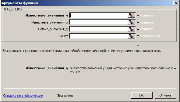
In "Excel" there is a function for calculating the value by OLS. It has the following form: “TREND” (known values of Y; known values of X; new values of X; const.). We apply the formula for calculating OLS in Excel to our table.
To do this, in the cell in which the result of the calculation by the least squares method is to be displayed in Excel, we enter the “=” sign and select the “TREND” function. In the window that opens, fill in the appropriate fields, highlighting:
- the range of known values for Y (in this case, data for turnover);
- range x 1 , ... x n , i.e., the size of the retail space;
- both known and unknown values of x, for which you need to find out the size of the turnover (information on their location on the worksheet see below).
In addition, in the formula there is a logical variable "Const". If you enter 1 in the corresponding field, then this will mean that calculations should be carried out, assuming that b = 0.
If you need to find out the forecast for more than one value of x, then after entering the formula, you should not click on “Enter”, but rather type on the keyboard the combination “Shift” + “Control” + “Enter”.
Some features
Regression analysis may be available even to dummies. The Excel formula for predicting the value of an array of unknown variables - "TREND" - can be used even by those who have never heard of the least squares method. Just know some of the features of her work. In particular:
- If you place the range of known values of the variable y in one row or column, then each row (column) with known values of x will be perceived by the program as a separate variable.
- If the “TREND” window does not specify a range with known x, then if you use the function in Excel, the program will consider it as an array of integers, the number of which corresponds to the range with the given values of the variable y.
- In order to get an array of “predicted” values at the output, the expression for calculating the trend needs to be entered as an array formula.
- If new x values are not specified, then the TREND function considers them equal to known. If they are not specified, then array 1 is taken as an argument; 2; 3; 4; ..., which is commensurate with the range with parameters y already set.
- A range containing new x values must consist of the same or more rows or columns as a range with given y values. In other words, it must be a proportionate independent variable.
- An array with known x values may contain several variables. However, if we are talking only about one, then it is required that the ranges with the given values of x and y be proportionate. In the case of several variables, it is necessary that the range with the given values of y fit in one column or in one row.
Predict function
Regression analysis in Excel is implemented using several functions. One of them is called “PREDICTION”. It is similar to "TRENDS", that is, it produces the result of calculations using the least squares method. However, only for one X for which the value of Y is unknown.
Now you know the formulas in Excel for dummies that allow you to predict the future value of a particular indicator according to a linear trend.