With matrices (tables with numerical elements) various computational actions can be carried out. One of them is multiplication by a number, a vector, another matrix, several matrices. The work sometimes turns out to be wrong. The erroneous result is the result of ignorance of the rules for performing computational actions. Let's see how to implement the multiplication.
Matrix and number
Let's start with the simplest thing - by multiplying the table with numbers by a specific value. For example, we have a matrix A with elements a ij (i are row numbers, and j are column numbers) and number e. The product of the matrix by e is the matrix B with elements b ij , which are found by the formula:
b ij = e × a ij .
That is, to get the element b 11 you need to take the element a 11 and multiply it by the desired number, to get b 12 you need to find the product of the element a 12 and the number e, etc.
We solve the problem number 1, presented in the picture. To get the matrix B, simply multiply the elements from A by 3:
- a 11 × 3 = 18. This value is written in the matrix B to the place where column No. 1 and row No. 1 intersect.
- a 21 × 3 = 15. We got the element b 21 .
- a 12 × 3 = –6. We got element b 12 . We write it in matrix B to the place where column No. 2 and row No. 1 intersect.
- a 22 × 3 = 9. This result is an element of b 22 .
- a 13 × 3 = 12. This number is entered in the matrix in place of the element b 13 .
- a 23 × 3 = –3. The last number received is the element b 23 .
Thus, we got a rectangular array with numeric elements.
Vectors and the condition for the existence of a product of matrices
In mathematical disciplines, there is such a thing as a “vector”. This term refers to an ordered set of values from a 1 to a n . They are called the coordinates of the vector space and are written in the form of a column. There is also the term "transposed vector." Its components are arranged as a string.
Vectors can be called matrices:
- a column vector is a matrix built from a single column;
- a row vector is a matrix that includes only one row.
When performing multiplication operations on matrices, it is important to remember that there is a condition for the existence of a product. The computational action A × B can be performed only when the number of columns in table A is equal to the number of rows in table B. The final matrix obtained as a result of the calculation always has the number of rows in table A and the number of columns in table B.
When multiplying, it is not recommended to interchange the matrices (factors). Their product usually does not correspond to the commutative (translational) law of multiplication, i.e., the result of the operation A × B is not equal to the result of the operation B × A. This feature is called the non-commutativity of the matrix product. In some cases, the result of multiplication A × B is equal to the result of multiplication B × A, i.e., the product is commutative. Matrices for which the equality A × B = B × A holds are called permutation. Examples of such tables can be found below.
Column Vector Multiplication
When performing matrix multiplication by a column vector, we must take into account the condition for the product to exist. The number of columns (n) in the table must match the number of coordinates that make up the vector. The result of the calculation is a transformed vector. Its number of coordinates is equal to the number of lines (m) from the table.
How are the coordinates of the vector y calculated if there is a matrix A and a vector x? For calculations, the formulas are created:
y 1 = a 11 x 1 + a 12 x 2 + ... + a 1 n x n ,
y 2 = a 21 x 1 + a 22 x 2 + ... + a 2n x n ,
………………………………………,
y m = a m1 x 1 + a m2 x 2 + ... + a mn x n ,
where x 1 , ..., x n are the coordinates from the x-vector, m is the number of rows in the matrix and the number of coordinates in the new y-vector, n is the number of columns in the matrix and the number of coordinates in the x-vector, a 11 , a 12 , ..., a mn are elements of the matrix A.
Thus, to obtain the ith component of the new vector, the scalar product is performed. From the matrix A, the ith row vector is taken, and it is multiplied by the existing vector x.
We solve problem No. 2. The product of the matrix by the vector can be found, because A has 3 columns, and x consists of 3 coordinates. As a result, we should get a column vector with 4 coordinates. We use the above formulas:
- We calculate y 1 . 1 × 4 + (–1) × 2 + 0 × (–4). The total value is 2.
- We calculate y 2 . 0 × 4 + 2 × 2 + 1 × (–4). In the calculation, we get 0.
- Calculate y 3 . 1 × 4 + 1 × 2 + 0 × (–4). The sum of the products of these factors is 6.
- Calculate y 4 . (–1) × 4 + 0 × 2 + 1 × (–4). The coordinate is –8.
Multiplying a row vector by a matrix
You cannot multiply a matrix consisting of several columns by a row vector. In such cases, the condition for the existence of the work is not satisfied. But the multiplication of a row vector by a matrix is possible. This computational operation is performed when the number of coordinates in the vector and the number of rows in the table match. The result of the product of the vector by the matrix is a new row vector. Its number of coordinates should equal the number of columns in the matrix.
The calculation of the first coordinate of the new vector implies the multiplication of the row vector and the first column vector from the table. The second coordinate is calculated in a similar way, but instead of the first column vector, the second column vector is taken. Here is a general formula for calculating coordinates:
y k = a 1 k x 1 + a 2 k x 2 + ... + a mk x m ,
where y k is the coordinate from the y-vector, (k is in the range from 1 to n), m is the number of rows in the matrix and the number of coordinates in the x-vector, n is the number of columns in the matrix and the number of coordinates in the y-vector, a with alphanumeric indices - elements of matrix A.
The product of rectangular matrices
This computational action may seem complicated. However, multiplication is easy to do. Let's start with the definition. The product of a matrix A with m rows and n columns and a matrix B with n rows and p columns is a matrix C with m rows and p columns, in which the element c ij is the sum of the products of the elements of the i-th row from table A and j-th a column from table B. In simpler terms, the element c ij is the scalar product of the ith row vector from table A and the jth column vector from table B.
Now we will understand in practice how to find the product of rectangular matrices. For this we solve problem No. 3. The condition for the existence of the product is satisfied. We proceed to the calculation of the elements c ij :
- Matrix C will consist of 2 rows and 3 columns.
- We calculate the element c 11 . To do this, we perform the scalar product of row No. 1 from matrix A and column No. 1 from matrix B. c 11 = 0 × 7 + 5 × 3 + 1 × 1 = 16. Then we proceed in a similar way, changing only rows and columns (depending on element index).
- c 12 = 12.
- c 1 3 = 9.
- c 21 = 31.
- c 22 = 18.
- c 2 3 = 36.
Elements are calculated. Now it remains only to compose a rectangular block of the obtained numbers.
Multiplication of three matrices: theoretical part
Is it possible to find the product of three matrices? This computational operation is doable. The result can be obtained in several ways. For example, there are 3 square tables (of the same order) - A, B and C. To calculate the product, you can:
- Multiply A and B first. Then multiply the result by C.
- First find the product of B and C. Next, multiply the matrix A by the result obtained.
If you want to multiply the rectangular matrix, then first you need to make sure that this computational operation is possible. There must be products A × B and B × C.
Phased multiplication is not a mistake. There is such a thing as “matrix multiplication associativity”. This term refers to the equality (A × B) × C = A × (B × C).
Multiplication of Three Matrices: Practice
Square matrices
Let's start by multiplying small square matrices. The figure below shows the task number 4, which we have to solve.
We will use the property of associativity. First we multiply either A and B, or B and C. We remember only one thing: you cannot interchange the factors, that is, you cannot multiply B × A or C × B. With this multiplication we get an erroneous result.
The course of the decision.
Step one. To find the common product, first we multiply A by B. When multiplying two matrices, we will be guided by the rules that were described above. So, the result of multiplying A and B will be a matrix D with 2 rows and 2 columns, i.e., a rectangular array will include 4 elements. Find them by doing the calculation:
- d 11 = 0 × 1 + 5 × 6 = 30;
- d 12 = 0 × 4 + 5 × 2 = 10;
- d 21 = 3 × 1 + 2 × 6 = 15;
- d 22 = 3 × 4 + 2 × 2 = 16.
The intermediate result is ready.
Step Two Now multiply the matrix D by the matrix C. The result should be a square matrix G with 2 rows and 2 columns. We calculate the elements:
- g 11 = 30 × 8 + 10 × 1 = 250;
- g 12 = 30 × 5 + 10 × 3 = 180;
- g 21 = 15 × 8 + 16 × 1 = 136;
- g 22 = 15 × 5 + 16 × 3 = 123.
Thus, the result of the product of square matrices is a table G with computed elements.
Rectangular Matrices
The figure below shows task No. 5. It is required to multiply rectangular matrices and find a solution.
Let us check whether the condition for the existence of the products A × B and B × C is fulfilled. The orders of the indicated matrices allow us to perform multiplication. We proceed to solve the problem.
The course of the decision.
Step one. Multiply B by C to get D. Matrix B contains 3 rows and 4 columns, and matrix C contains 4 rows and 2 columns. This means that we get the matrix D with 3 rows and 2 columns. Calculate the elements. Here are 2 calculation examples:
- d 11 = 3 × 0 + 0 × 0 + 1 × 0 + 0 × 1 = 0;
- d 1 2 = 3 × 2 + 0 × 3 + 1 × 1 + 0 × 6 = 7.
We continue to solve the problem. As a result of further calculations, we find the values of d 2 1 , d 2 2 , d 31 and d 32 . These elements are 0, 19, 1, and 11, respectively. We write the found values into a rectangular array.
Step Two Multiply A by D to get the final matrix F. It will have 2 rows and 2 columns. We calculate the elements:
- f 11 = 2 × 0 + 6 × 0 + 1 × 1 = 1;
- f 12 = 2 × 7 + 6 × 19 + 1 × 11 = 139;
- f 21 = 0 × 0 + 1 × 0 + 3 × 1 = 3;
- f 22 = 0 × 7 + 1 × 19 + 3 × 11 = 52.
We compose a rectangular array, which is the final result of the multiplication of three matrices.
Acquaintance with the direct work
The material that is quite difficult to understand is the Kronecker product of matrices. It has an additional name - a direct work. What is meant by this term? Suppose we have a table A of order m × n and a table B of order p × q. The direct product of matrix A by matrix B is a matrix of order mp × nq.
We have 2 square matrices A, B, which are shown in the picture. The first of them consists of 2 columns and 2 rows, and the second of 3 columns and 3 rows. We see that the matrix obtained as a result of the direct product consists of 6 rows and exactly the same number of columns.
How does the direct product calculate the elements of a new matrix? Finding the answer to this question is very easy if you analyze the picture. First fill in the first line. Take the first element from the top row of table A and sequentially multiply by the elements of the first row from table B. Next, take the second element of the first row of table A and sequentially multiply by the elements of the first row of table B. To fill the second row, again take the first element from the first row of table A and multiply it by the elements of the second row of table B.
The final matrix obtained by the direct product is called the block matrix. If we re-analyze the figure, we can see that our result consists of 4 blocks. All of them include elements of matrix B. Additionally, the element of each block is multiplied by a specific element of matrix A. In the first block, all elements are multiplied by a 11 , in the second - on a 12 , in the third - on a 21 , in the fourth - on a 22 .
Key to a work
When considering the topic of matrix multiplication, it is worth considering a term such as “determinant of the product of matrices”. What is a qualifier? This is an important characteristic of a square matrix, a certain value that is put in correspondence with this matrix. The determinant letter is det.
For a matrix A consisting of two columns and two rows, the determinant is easy to find. There is a small formula, which is the difference between the products of specific elements:
det A = a 11 × a 22 - a 12 × a 21 .
Consider an example of calculating the determinant for a second-order table. There exists a matrix A in which a 11 = 2, a 12 = 3, a 21 = 5 and a 22 = 1. To calculate the determinant, we use the formula:
det A = 2 × 1 - 3 × 5 = 2 - 15 = –13.
For 3 × 3 matrices, the determinant is calculated by a more complex formula. It is presented below for matrix A:
det A = a 11 a 22 a 33 + a 12 a 23 a 31 + a 13 a 21 a 32 - a 13 a 22 a 31 - a 11 a 23 a 32 - a 12 a 21 a 33 .
To memorize the formula, they came up with the triangle rule, which is illustrated in the picture. First, the elements of the main diagonal are multiplied. To the obtained value are added the products of those elements that are indicated by the angles of triangles with red sides. Next, the product of the elements of the side diagonal is taken away and the products of those elements indicated by the angles of the triangles with the blue sides are taken away.
Now let's talk about the determinant of the product of matrices. There is a theorem that states that this indicator is equal to the product of the determinants of the factor tables. We will verify this with an example. We have a matrix A with elements a 11 = 2, a 12 = 3, a 21 = 1 and a 22 = 1 and a matrix B with elements b 11 = 4, b 12 = 5, b 21 = 1 and b 22 = 2 Find the determinants for the matrices A and B, the product A × B, and the determinant of this product.
The course of the decision.
Step one. We calculate the determinant for A: det A = 2 × 1 - 3 × 1 = –1. Next, we calculate the determinant for B: det B = 4 × 2 - 5 × 1 = 3.
Step Two Find the product A × B. We denote the new matrix by the letter C. Let us calculate its elements:
- c 11 = 2 × 4 + 3 × 1 = 11;
- c 1 2 = 2 × 5 + 3 × 2 = 16;
- c 2 1 = 1 × 4 + 1 × 1 = 5;
- c 22 = 1 × 5 + 1 × 2 = 7.
Step Three We calculate the determinant for C: det C = 11 × 7 - 16 × 5 = –3. Compare with the value that could be obtained by multiplying the determinants of the original matrices. The numbers are the same. The above theorem is true.
Product Rank
The rank of a matrix is a characteristic that reflects the maximum number of linearly independent rows or columns. To calculate the rank, elementary matrix transformations are performed:
- rearrangement of two parallel rows;
- multiplication of all elements of a certain series from the table by a number that is not equal to zero;
- adding to elements of one row of elements from another row multiplied by a specific number.
After elementary transformations, look at the number of non-zero rows. Their number is the rank of the matrix. Consider the previous example. It presented 2 matrices: A with elements a 11 = 2, a 12 = 3, a 21 = 1 and a 22 = 1 and B with elements b 11 = 4, b 12 = 5, b 21 = 1 and b 22 = 2. We will also use the matrix C obtained as a result of multiplication. If we perform elementary transformations, then there will be no zero rows in the simplified matrices. This means that the rank of table A, and the rank of table B, and the rank of table C is 2.
Now we will pay special attention to the rank of the product of matrices. There is a theorem which states that the rank of a product of tables containing numeric elements does not exceed the rank of any of the factors. This can be proved. Let A be a k × s matrix and B be an s × m matrix. The product of A and B is C.
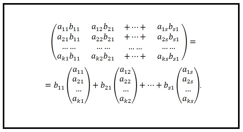
We study the picture presented above. It shows the first column of the matrix C and its simplified notation. This column is a linear combination of the columns included in the matrix A. Similarly, we can say about any other column from the rectangular array C. Thus, the subspace formed by the column vectors of table C exists in the subspace formed by the column vectors of table A. for this reason, the dimension of subspace No. 1 does not exceed the dimension of subspace No. 2. It follows from this that the rank in the columns of table C does not exceed the rank in the columns of table A, that is, r (C) ≤ r (A). If we reason in the same way, we can verify that the rows of the matrix C are linear combinations of the rows of the matrix B. This implies the inequality r (C) ≤ r (B).
How to find a product of matrices is a rather complicated topic. It can be easily mastered, but to achieve such a result, you will have to devote a lot of time to memorizing all existing rules and theorems.